General Matrix Multiply (GEMM) is the core operation of neural networks. Whether you're running a large language model or a vision transformer, almost everything eventually reduces to matrix multiplication.
At its core, GEMM computes each output element as a dot product:
In this post, I'll walk through GEMM in C++ starting from a naive implementation and gradually building optimized versions.
What exactly are FLOPs?
FLOPs stands for Floating Point Operations. It's simply a count of how many arithmetic operations (mainly multiplications and additions) are required to perform a computation.
FLOPs don't tell you everything about performance, but they give a very useful baseline for understanding why matrix multiplication scales the way it does.
Alright, let's take a 2x2 matrix and try to calculate FLOPS by hand.
Step 1
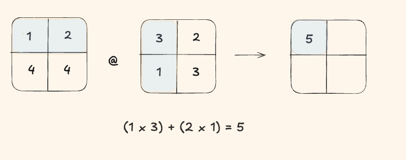
To compute the first output element, we performed:
- 2 multiplications
- 1 addition
That's a total of 3 FLOPs for a single output element.
Okay one more, just to be sure.
Step 2
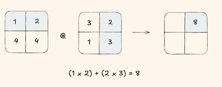
We again did 2 multiplies + 1 add = 3 FLOPs.
Since a 2x2 output matrix has 4 elements:
Total FLOPs = 4 × 3 = 12
For an \(N \times N\) matrix multiplication:
- Output matrix has \(N^2\) elements
- Each element performs \(N\) multiplications
- Each element performs \(N - 1\) additions
- Total operations per element: \(N + (N - 1) \approx 2N\)
Optimization Logbook
This is a series of implementations of GEMM in C++, each building on the previous with targeted optimizations. Benchmarks are measured on a Mac M4 Air (10 core CPU) multiplying two \(2048 \times 2048\) matrices. The compiler used is g++ with no optimization flags to isolate the effects of each code change.
Note* I use 1D arrays with stride based indexing to represent 2D matrices. The element at [i][j] is accessed as array[i * stride + j]
1. Naive Implementation
the most natural way to perform matrix multiplication is the triple nested loop.
for(int i = 0; i < rows; i++){
    for(int j = 0; j < cols; j++){
      int sum = 0;
      for(int k = 0; k < cols; k++){
        sum += M[i * stride + k] * N[k * stride + j];
        O[i * stride + j] = sum;
    }
  }
}
Performance:
- Runtime: \(34,500\) ms
- Total FLOPs: \(17.2\) GFLOPs
2. Register Optimization
take a look at this line O[i * stride + j] = sum; do you notice something wrong about where it is placed?
In the naive implementation, for every single multiplication and addition operation,
we're also performing a memory write to O[i * stride + j].
What if we move the write outside the innermost loop. Now sum accumulates in a CPU register, and we only write the final result to memory once per output element.
for(int i = 0; i < rows; i++){
    for(int j = 0; j < cols; j++){
      int sum = 0;
      for(int k = 0; k < cols; k++){
        sum += M[i * stride + k] * N[k * stride + j];
      }
      O[i * stride + j] = sum;  // moved outside the k loop
    }
  }
Performance:
- Runtime: \(26,520\) ms
- Speedup: \(1.3\times\) faster
Easy gains!
3. Loop Reordering
The previous optimizations helped, but we're still thrashing the cache. Our memory access pattern jumps around randomly instead of reading sequentially.
Understanding Cache Lines
The data is stored in memory sequentially row by row (row major order). When the CPU requests a single byte from memory, it doesn't just load that byte, it loads an entire cache line (typically 64 bytes). If your next memory access is nearby, great! If not, you've wasted that entire cache line.
In our register optimized version with loop order ijk, look at what happens:
for(int i = 0; i < N; i++){
    for(int j = 0; j < N; j++){
      int sum = 0;
      for(int k = 0; k < N; k++){
        sum += M[i * N + k] * N[k * N + j];  // N[k * N + j] jumps by N each time!
      }
      O[i * N + j] = sum;
    }
}- The access pattern for matrix \(M\) is: \(M[i*N+0]\), \(M[i*N+1]\), \(M[i*N+2]\)... We're accessing row \(i\) sequentially, which is great for cache locality.
- The access pattern for matrix \(N\) is: \(N[0*N+j]\), \(N[1*N+j]\), \(N[2*N+j]\)... We're accessing column \(j\), jumping by \(N\) elements (e.g. \(2048\) x \(4\) bytes = \(8\)KB) each iteration. This completely misses the cache, we load a \(64\) byte cache line but only use \(4\) bytes from it!
The solution is to reorder the loops to ikj:
for(int i = 0; i < rows; i++){
    for(int k = 0; k < cols; k++){ // 'k' moved to the middle
        int temp_M = M[i * stride + k]; // load once, use for the whole 'j' loop
        for(int j = 0; j < cols; j++){ // 'j' is now the innermost
            O[i * stride + j] += temp_M * N[k * stride + j];
        }
    }
}
Performance:
- Runtime: \(8,000\) ms
- Total speedup: \(4.3\) times faster than naive implementation
4. Compiler Flags
Our final optimization involves using compiler flags to enable automatic optimizations:
-
-O3enables high level optimizations such as function inlining, loop unrolling, and vectorization. -
-march=nativeallows the compiler to use CPU specific instructions for my architecture. -
-ffast-mathenables a range of optimizations that provide faster, though sometimes less precise, mathematical operations.
Performance:
- Runtime: \(527\) ms
- Total speedup: \(65\) x faster!
Conclusion
| Optimization | Runtime (ms) | Speedup |
|---|---|---|
| 1. Naive Implementation | \(34,500\) | \(1.0\)× |
| 2. Register Optimization | \(26,520\) | \(1.3\)× |
| 3. Loop Reordering | \(8,000\) | \(4.3\)× |
| 4. Compiler Flags | \(527\) | \(65\)× |
While this implementation is significantly faster, there are still many techniques to further improve this using tiling, SIMD vectorization, and parallelization.