Torch Internals (Part 3) - AOT Autograd

In the last two posts, we saw how torch.fx turns python code into a graph using symbolic tracing, and how TorchDynamo captures graphs at the bytecode level. But both only capture the forward pass. What about the backward pass?

Before the torch.compile ecosystem, users could capture the forward graph using torch.fx tracing, but the backward was still generated by the autograd engine dynamically, and the compiler can only see the forward graph. This means you could not merge the forward and backward computation graphs into a single graph to optimize across the boundary.

AOTAutograd solves exactly this. It traces both forward and backward ahead of execution and the compiler can now apply optimizations to the entire graph as a whole.

aot_function

Let's start with the simplest possible example using aot_function from functorch.compile. We define a function that multiplies two tensors, then wrap it with a compiler that just prints the graph:

import torch
from functorch.compile import aot_function, make_boxed_func

def fn(a, b):
    return a * b

def compiler_fn(fx_module, _):
    print(fx_module.code)
    return make_boxed_func(fx_module.forward)

a, b = [torch.randn(2, 4, requires_grad=True, device="cuda")
        for _ in range(2)]

aot_fn = aot_function(fn, fw_compiler=compiler_fn,
                      bw_compiler=compiler_fn)
res = aot_fn(a, b)
loss = res.sum()
loss.backward()

This prints two graphs - the forward and the backward. Let's read them carefully

def forward(self, primals_1, primals_2):
    mul = torch.ops.aten.mul.Tensor(primals_1, primals_2)
    return (mul, primals_1, primals_2)

What is a primal? primals are the original inputs to the function or in autograd terminology, primals are the tensors you apply an operation to. Here primals_1 = a and primals_2 = b.

The forward returns (mul, primals_1, primals_2) Why are we returning three values?. The first is the actual output (a * b). The other two tensors are saved for backward.

Let's look at the backward graph now.

def forward(self, primals_1, primals_2, tangents_1):
    mul_1 = torch.ops.aten.mul.Tensor(tangents_1, primals_1)
    mul_2 = torch.ops.aten.mul.Tensor(tangents_1, primals_2)
    return (mul_2, mul_1)

The first two parameters primals_1, primals_2 are the saved tensors from the forward pass. tangents are simply the incoming gradients you calculate during the backward pass.

The backward returns (mul_2, mul_1) gradients in the same order as the forward's original inputs (a, b). This ordering contract is how autograd knows which gradient belongs to which parameter.

Why AOT?

Normally, PyTorch's autograd builds the backward graph dynamically during forward propagation. The backward graph is only finalized once forward finishes. This is flexible, but you never get to see the full graph before execution.

AOTAutograd does this differently. It traces both forward and backward propagation Ahead-of-Time, before the function is actually executed. This gives you both computation graphs upfront.

Here is the general workflow:

1. AOT Dispatch traces forward and backward and generates a joint graph which is basically a FX graph containing Aten/Prim operators for both forward and backward.
2. Partition divides the joint graph into separate forward and backward graphs using partition_fn.
3. Optional decomposition where high-level operators are broken down to smaller granular operators.
4. The separate graphs are compiled and integrated into one torch.autograd.Function.

torch dispatcher

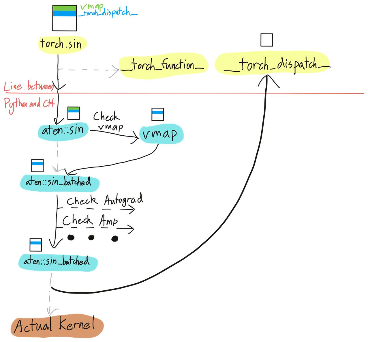
PyTorch has a dispatcher that you can think of like a router. Every time you call an operator like a * b, the dispatcher decides which kernel to run based on the input tensors' properties. CUDA tensor? Run the CUDA kernel. Needs gradients? Wrap it with autograd. An operator usually passes through multiple dispatch layers before reaching the final kernel.

__torch_dispatch__ is a hook that fires before the final kernel executes. It gives you access to the raw ATen operator and its inputs so you can intercept, inspect, or modify behavior at the op level.

make_fx

torch.fx has something called make_fx, which unlike regular symbolic_trace, is implemented through __torch_dispatch__. This gives it access to low-level ATen operators.

Take a look at the example below.

import torch
from torch.fx.experimental.proxy_tensor import make_fx


def f(x, y):
    return x + y

x = torch.randn(8)
y = torch.randn(8)

g = make_fx(f)(x, y)
print(g.code)

def forward(self, x_1, y_1):
    add = torch.ops.aten.add.Tensor(x_1, y_1)
    return add

from torch.fx import symbolic_trace
h = symbolic_trace(f)
print(h.code)

def forward(self, x, y):
    add = x + y
    return add

Okay perfect, now that we have seen why torch dispatcher is important, we can move onto joint graphs and how to create them.

The Joint Graph

The idea of having a single FX graph covering both forward and backward gives us the potential to optimize across the entire boundary instead of looking at forward and backward separately.

Here's the idea in pseudocode.

def joint_forward_backward(*inputs):
    outputs = forward_fn(*inputs)
    grads = torch.autograd.grad(
        outputs, inputs, grad_outputs=...
    )
    return outputs, grads

During tracing, every operator is intercepted by __torch_dispatch__ and for each operator, AOTAutograd -

1. Retrieves the FX proxy from the tensor.
2. Creates a call_function node in the FX graph with the ATen operator as target.
3. Runs the operator with the actual tensor.
4. Binds the resulting tensor to the proxy.

This repeats until AOTAutograd has traced all operators in both forward and backward propagation, producing a complete joint graph.

Partitioning the Joint Graph

Once we have the joint graph, we need to split it back into separate forward and backward graphs. AOTAutograd's partition_fn does this, and has two built-in strategies. Let's compare them with a concrete example:

def fn(a, b, c, d):
    x = a + b + c + d
    return x.cos().cos()

default_partition

This is the default behavior we saw in the first example where we finds all operator outputs from input to forward output. The tensors that are needed for the backward are also included as forward outputs and all the intermediate results are preserved.

def forward(self, primals_1, primals_2, primals_3, primals_4):
    add   = torch.ops.aten.add.Tensor(primals_1, primals_2)
    add_1 = torch.ops.aten.add.Tensor(add, primals_3)
    add_2 = torch.ops.aten.add.Tensor(add_1, primals_4)
    cos   = torch.ops.aten.cos.default(add_2)
    cos_1 = torch.ops.aten.cos.default(cos)
    return (cos_1, add_2, cos)    # saves add_2 and cos for backward

The backward receives these saved tensors as inputs

def forward(self, add_2, cos, tangents_1):
    sin   = torch.ops.aten.sin.default(cos)
    neg   = torch.ops.aten.neg.default(sin)
    mul   = torch.ops.aten.mul.Tensor(tangents_1, neg)
    sin_1 = torch.ops.aten.sin.default(add_2)
    neg_1 = torch.ops.aten.neg.default(sin_1)
    mul_1 = torch.ops.aten.mul.Tensor(mul, neg_1)
    return (mul_1, mul_1, mul_1, mul_1)

Background: Memory bound operations

This is a background section to help motivate the next technique and why it works so well.

If you remember on GPUs, the majority of time spent on an operator is not the arithmetic, but actually memory reads and writes. This is especially true for pointwise operators (add, mul, cos, sin, relu, etc.), which do very little compute per element.

So fusing multiple pointwise ops might not help at all since the bottleneck is the memory access, not the flops.

Now in training, if your graph is a chain of pointwise ops, both forward and backward are entirely pointwise and the runtime is proportional to the amount of memory you read and write. Since the default partition saves every intermediate tensor, you're essentially paying the memory cost twice (save in forward, load in backward).

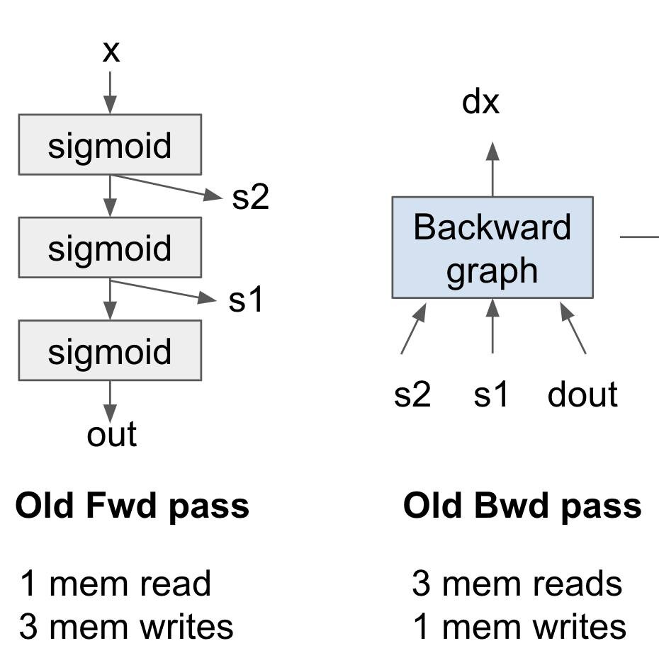
What if you instead save only the input and recompute the intermediates in backward? This means -

1. fewer tensors saved between forward and backward.
2. and reduced memory accesses since we have no writes to save intermediates and no reads to load them back.

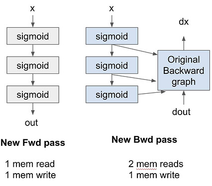
The recompute itself is essentially free because those pointwise ops are already memory-bound and the extra flops are okay since they hide behind the memory latency. This is what makes activation checkpointing work, and AOTAutograd generalizes it with a min-cut formulation.

min_cut_rematerialization_partition

Cool, now that we have laid out that we don't need to save all the intermediate tensors, how do we decide between what to save vs what to recompute. This is framed as a max-flow/min-cut problem (You can read on this algorithm later).

Let's look at the same code with the min-cut partitioner:

from functorch.compile import min_cut_rematerialization_partition

aot_fn = aot_function(fn, fw_compiler=compiler_fn,
                      bw_compiler=compiler_fn,
                      partition_fn=min_cut_rematerialization_partition)

Look at the forward graph and note that cos is no longer saved:

def forward(self, primals_1, primals_2, primals_3, primals_4):
    add   = torch.ops.aten.add.Tensor(primals_1, primals_2)
    add_1 = torch.ops.aten.add.Tensor(add, primals_3)
    add_2 = torch.ops.aten.add.Tensor(add_1, primals_4)
    cos   = torch.ops.aten.cos.default(add_2)
    cos_1 = torch.ops.aten.cos.default(cos)
    return (cos_1, add_2)    # only saves add_2, NOT cos

Now in the backward graph cos is recomputed from add_2 instead of being saved.

def forward(self, add_2, tangents_1):
    cos   = torch.ops.aten.cos.default(add_2)  # recomputed!
    sin   = torch.ops.aten.sin.default(cos)
    neg   = torch.ops.aten.neg.default(sin)
    mul   = torch.ops.aten.mul.Tensor(tangents_1, neg)
    sin_1 = torch.ops.aten.sin.default(add_2)
    neg_1 = torch.ops.aten.neg.default(sin_1)
    mul_1 = torch.ops.aten.mul.Tensor(mul, neg_1)
    return (mul_1, mul_1, mul_1, mul_1)

Wrapping Up

Great job if you made it this far! In the next post, we will look at the final piece of the entire stack which is TorchInductor and see how the captured graphs and lowered into efficient triton code.